Political GPS

Political GPS is a program that uses real-time GPS data to display the electoral district you are in and the political party in power. Election results and geographic boundary data are stored locally, so no internet connection is required.

Optimized to run on a Raspberry Pi Zero W with 16x2 LCD RGB backlit display and Adafruit Ultimate GPS module.


Political GPS Display

Motivation:

Driving around during an election, the political lean of different parts of the country becomes readily apparent due to the abundance of political signage. Huge differences in political affiliation can be observed between neighborhoods that appear otherwise identical. However, when the election ends and yard signs, banners, and flags are taken down, these political differences become far less visible.

I was interested making a tool that revealed these hidden political affiliations as I drove through different neighborhoods.

Process:

Election data:

Living in Canada, I decided to use the results of the most recent Canadian election, which at the time was the 2015 federal election. Geographic boundary data for all 338 federal districts were available on the Canadian government website as a shapefile (.shp). Election results by federal district were also available and were added to the shapefile using GIS software (QGIS).


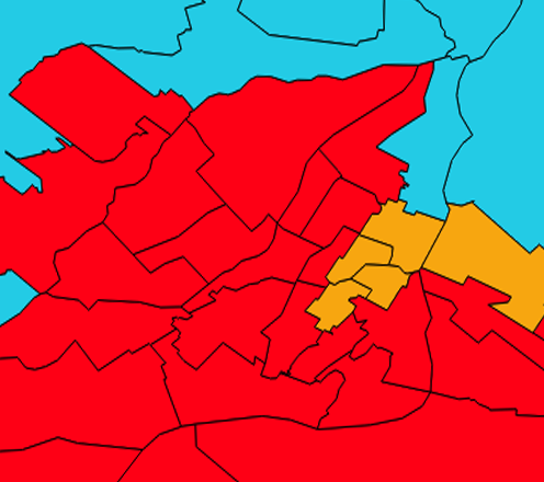
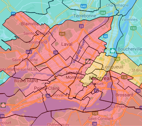
Montreal Districts (party by color)	Map Overlay

District location:

Next, I needed a way to determine if my latitude/longitude coordinate was in a particular district. As districts were represented by arrays of vertices, this was a point-in-polygon problem which I solved using the ray casting (aka crossing number) algorithm. With this, I was able to find my current district by checking each district sequentially.

However, there was a problem with several districts that completely encompassed smaller districts (enclaves). These encompassing districts were each defined by multiple polygons. A single outer “donut” and one or more inner “donut holes” or, given that these are Canadian districts, “Timbits”. If I was located inside one of these holes and I only checked the outer donut polygon, I would wrongfully assume I was in the encompassing district rather than the enclave.


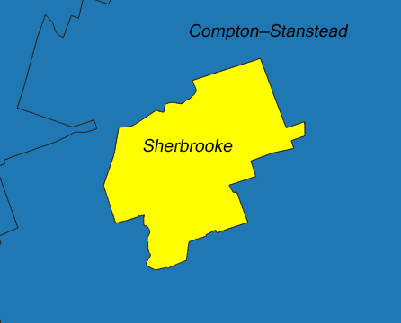
Enclave district

I solved this problem by first checking whether my location was located in any of the few enclave districts. Once enclaved districts were ruled out, I could check just the outer polygons of the remaining districts without issue.

Optimization

While checking every district sequentially runs quickly on a desktop, it was far too inefficient to run on a Pi Zero. Each point-in-polygon check only has a time complexity of O(n) where n is the number of vertices, but because of the large number of vertices and hundreds of districts to check, it was still very slow. If the number of vertices was reduced, I could improve performance proportionally.

The geographic data was extremely detailed with over 500,000 vertices. As this level of granularity, down to the meter, wasn’t required for the project, I was able to simplify the geometry. Using the Douglas-Peucker algorithm , I was able to remove 90% of the vertices while still maintaining fine geometric detail.


Simplified	Simplified (Vertices)

The geometry simplification certainly helped by significantly decreasing the time required to search each district, but district localization was still too slow. I decided the best way to reduce the number of districts that needed to be searched was to sort the districts by proximity. Specifically, how far my current position was to the center (centroid) of each district. Using QGIS, I computed the centroid of each district polygon and added it to my dataset.


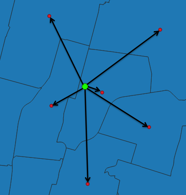
Distance to district center

Calculating the distance between my current position and the centroid of each district was extremely quick. Sorting districts by proximity has a time complexity of O(n log n) using Python’s Timsort method. However, following the first sort, the order of districts by proximity remains largely stable and only requires limited sorting. This meant that, on average, I only had to check the closest 1-2 districts each time.

Together, the optimization from reducing the total vertices and proximity sorting districts was enough that the program could run using real-time GPS data on a Pi Zero.

Hardware:

Parts:


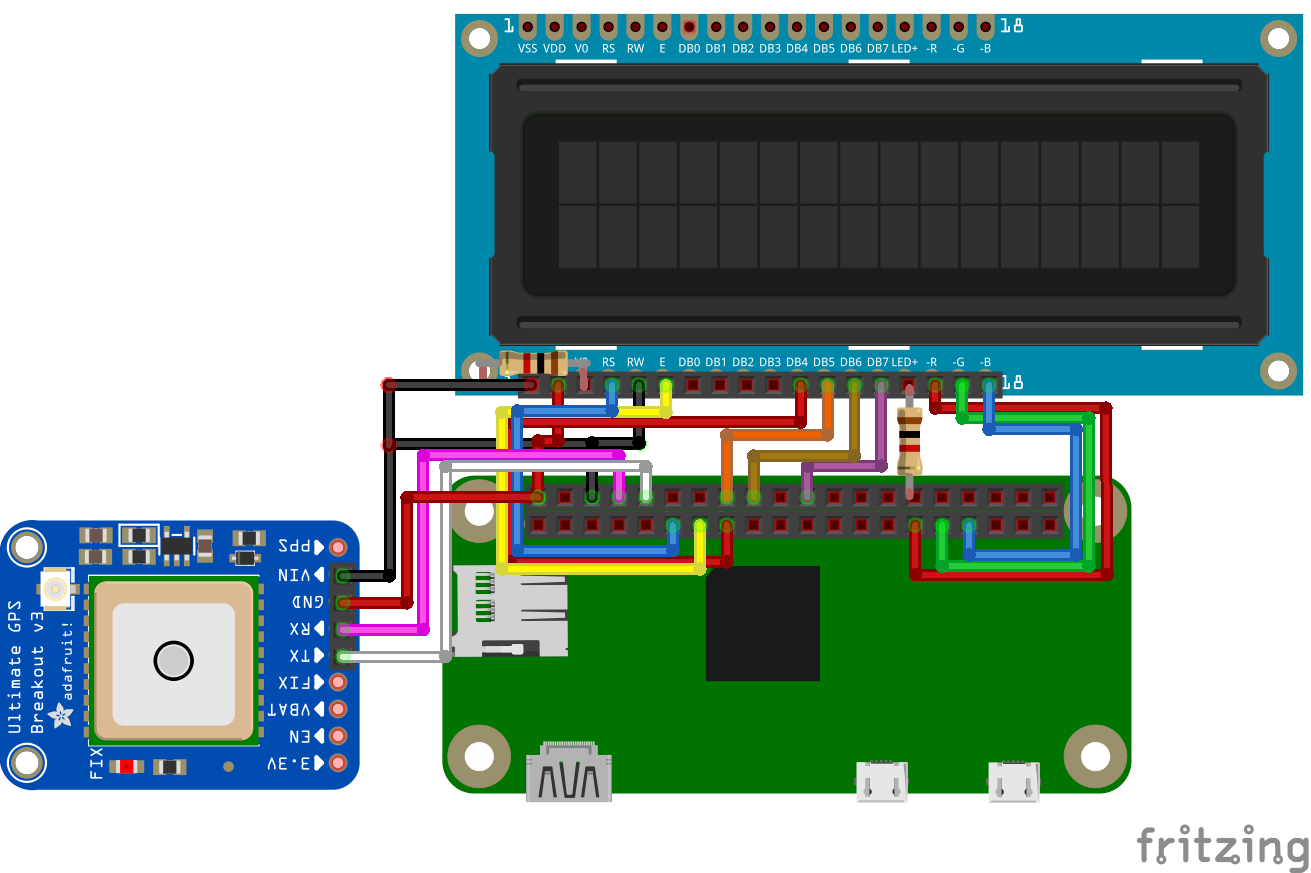Wiring between components

Built using:

QGIS for geographic data processing
gps3 for reading real-time GPS data
digitalio/adafruit_character_lcd for controlling LCD display
pigpio for hardware timed PWM to control color of RGB backlight